I’ve long been wondering how much power my Homelab consumes, especially with my switch from a single relatively beefy server to a gaggle of Raspberry Pis.
In the end, I put in three smart plugs supporting MQTT. I would have loved to have per-machine power consumption stats, but I didn’t want to invest that much money into smart plugs.
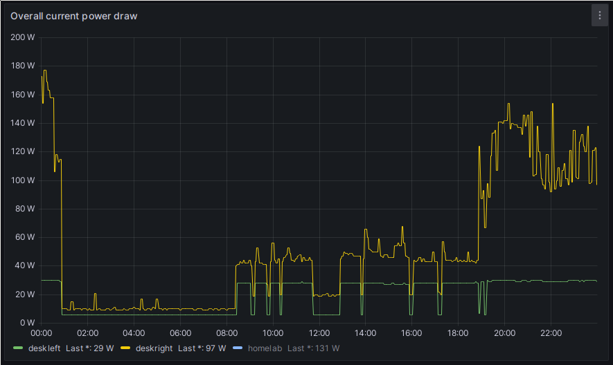
To wet your appetite a bit, here is a snapshot of the resulting Grafana dashboard:
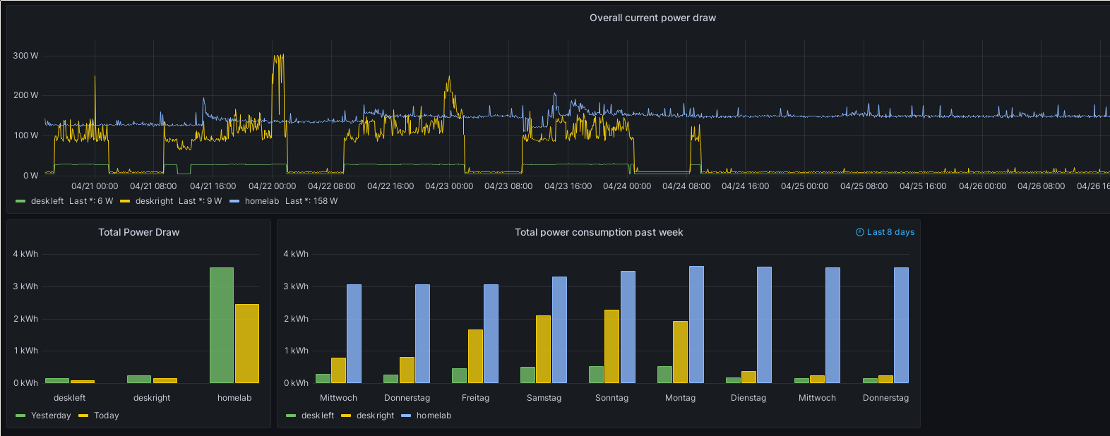
Screenshot of my power consumption dashboard.
These plots are produced from two of the data points provided by my smart plugs, namely the total current power draw, and the total daily consumption in kWh. I will go into more detail on the plots later in this article.
I will show the setup of the Tasmota based smart plugs I bought. In addition, I’m using Mosquitto as my MQTT message broker. The mqtt2prometheus exporter does the conversion of MQTT messages from the plugs to the prometheus format.
Here is an overview of the setup:

Overview of the power measurement setup. The red arrows mark the IoT VLAN, and the blue arrows mark the Homelab VLAN.
After the setup, I will also give an overview of the information I got out of this, to show the utility of a setup like this.
One question you might already have is: Why not Home Assistant? The answer is pretty simple: I’ve got no plans, at the moment at least, to go any further than using the plugs to measure power consumption. There’s going to be no automation. So Home Assistant would be overkill for my purpose. If and when I start using automations, I will reconsider. But for now, I’m pretty happy with my “several tools doing one thing right approach”, instead of Home Assistant’s Swiss Army knife approach.
Setting up an IoT WiFi
As I noted in a previous post, I already have a VLAN for my IoT devices. Until I installed the plugs, it was only home to my VOIP DECT base station and my network printer.
Now, I need to extend that VLAN to a separate WiFi in my OpenWRT WiFi router.
The first step in doing so is to actually configure an additional WiFi for the plugs.
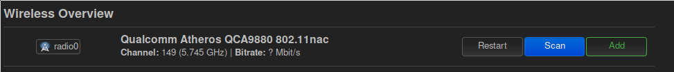
Screenshot of the radio entry in the OpenWRT device list.
Adding an additional WiFi in OpenWRT is pretty simple. Just chose the radio you want to use in your device list (I’ve got two for example, the 2.4 GHz and the 5 GHz one). Then click the “Add” button, and a new window for configuring the new WiFi will appear.
One important note: I’m not 100% sure whether supporting multiple WiFis at once is the default now, or whether it depends on the WiFi chipset any given AP uses. So check yours to make sure before embarking on a big project. 😉
I gave the new WiFi a catchy name (okay, I just appended “iot” to my existing WiFi’s name 😅) and then hid the SSID. This isn’t a security measure, it just relieves the WiFi clutter a bit by hiding a WiFi which is not intended to ever be used by humans.
One thing I found important to do: Enabling the “Isolate Clients” option in the “Advanced Settings” tab. This prevents two clients on that WiFi from talking to each other. My IoT devices will get to talk to exactly one thing, my MQTT broker, and absolutely nothing else.
Next up is configuring the new WiFi to use the IoT VLAN. I will not go into details here, as I’ve already detailed the setup for a WiFi VLAN in my detailed article on VLANs, and there were no special configs required for the IoT VLAN. The only thing to mention on this is that the IoT VLAN is pretty much nailed shut. The only outgoing connections allowed are to the Firewall itself, for DHCP and DNS, and to the MQTT broker.
The plugs
The plugs I bought were from Athom. The main draw was the relatively low cost, and the fact that they already come with Tasmota pre-flashed. They also support a sufficiently high max load of 3680 Watts.
The advantage of using Tasmota is that it is an Open Source firmware, that requires some configuration for different devices - but not individual rebuilds. It’s also independent of the vendor, which means I don’t have to care at all whether the manufacturer continues to support them or not. The plugs also have an industry standard SoC, the ESP8266.
So in short: No cloud required! (Well, besides your own internal cloud, depending on the size of your Homelab. 😉)
They are WiFi connected, which makes deployment a bit easier, with no new networking equipment for e.g. Zigbee needed.
When first starting a fresh plug, or after resetting it, Tasmota starts the WiFi chip in AP mode, so you can connect with your phone or another WiFi device. Then it shows a website for configuring the WiFi the plug should be connecting to.
After doing that configuration, the plug’s MQTT settings also need to be configured. But first we need to set up an MQTT broker - and explain what MQTT even is.
Finally, a modest amount of security. Tasmota supports Basic Auth, which I have set up to secure the Web UI. Go to “Configuration” -> “Configure Other” and enter a password under “Web Admin Password”.
MQTT
Not having worked with MQTT ever before, I found this series on it a pretty good introduction.
In principle, MQTT (Message Queuing Telemetry Transport) is a protocol for transmitting metrics. It is kept deliberately simple, so that it can be implemented easily on the low power chips of IoT devices.
MQTT is a pub/sub system. You’ve got a central broker. Clients can then connect to that broker and subscribe to topics, like “power_plugs/living_room/plug3” or just “power_plugs” to receive all events other devices push to that topic. In my setup, the Tasmota power plugs push to topics called plugs/tasmota/tele.
The messages pushed by MQTT clients are in JSON format. A message from the plugs looks like this:
{
  "Time": "2023-06-08T22:01:44",
  "ENERGY": {
    "TotalStartTime": "2023-02-01T21:57:12",
    "Total": 405.918,
    "Yesterday": 3.481,
    "Today": 3.19,
    "Period": 12,
    "Power": 150,
    "ApparentPower": 214,
    "ReactivePower": 153,
    "Factor": 0.7,
    "Voltage": 233,
    "Current": 0.918
  }
}
This is a message from my Homelab plug. The lab currently draws around 150 W, at my local ~230 V, and today I had already used 3.19 kWh.
An MQTT broker can be observed with several tools, which can subscribe to all or a subset of messages. I’ve found MQTT Explorer to be working well for manual monitoring.
The plugs are also subscribed to specific topics. By publishing certain messages to those topics, the plugs can for example be switched on and off. As I mentioned above, I’m not doing any automation, only energy consumption measurement, so I’m not using that feature at the moment.
From a security standpoint, MQTT supports user credentials and working over TLS. More on those topics when I go over the Mosquitto setup.
Setting up the MQTT broker
I’m using Mosquitto as my MQTT broker. Main reason: It’s open source, and it was mentioned by a lot of the other IoT open source tools I’ve been using.
It has an official Docker container here. As always, I’m deploying it in my Nomad cluster, with the following job config:
job "mosquitto" {
  datacenters = ["homenet"]

  priority = 50

  constraint {
    attribute = "${node.class}"
    value     = "internal"
  }

  group "mosquitto" {

    network {
      mode = "bridge"
      port "mqtt" {}
    }

    service {
      name = "mosquitto"
      port = "mqtt"

      tags = [
        "traefik.enable=true",
        "traefik.tcp.routers.mosquitto.entrypoints=mqtt",
        "traefik.tcp.routers.mosquitto.rule=HostSNI(`*`)",
        "traefik.tcp.routers.mosquitto-tls.entrypoints=my-entry",
        "traefik.tcp.routers.mosquitto-tls.rule=HostSNI(`mqtt.example.com`)",
        "traefik.tcp.routers.mosquitto-tls.tls=true",
      ]
    }

    volume "vol-mosquitto" {
      type            = "csi"
      source          = "vol-mosquitto"
      attachment_mode = "file-system"
      access_mode     = "single-node-writer"
    }

    task "mosquitto" {
      driver = "docker"

      config {
        image = "eclipse-mosquitto:2.0.15"

        mount {
          type = "bind"
          source = "local/conf/"
          target = "/mosquitto/config"
        }
      }

      volume_mount {
        volume      = "vol-mosquitto"
        destination = "/mosquitto/data"
      }

      vault {
        policies = ["mosquitto"]
      }

      dynamic "template" {
        for_each = fileset(".", "mosquitto/conf/*")
        content {
          data = file(template.value)
          destination = "local/conf/${basename(template.value)}"
          perms = "600"
        }
      }

      template {
        data = file("mosquitto/templates/passwd")
        destination = "secrets/passwd"
        change_mode = "restart"
        perms = "600"
      }

      template {
        data = file("mosquitto/templates/mosquitto.conf")
        destination = "local/conf/mosquitto.conf"
        change_mode = "restart"
        perms = "600"
      }

      resources {
        cpu = 100
        memory = 50
      }
    }
  }
}
I’ve cut a couple of tasks out of the above config, as they pertain to the Prometheus exporters for the MQTT data. I will go into detail about them later.
As I always do, I’m putting the service into a bridge network.
But in contrast
to my normal usage of Consul Connect networking to connect services, I’m using
an exposed port, mqtt, here. The reason for this is that MQTT is a pure TLS/TCP
protocol. And these don’t currently work together with Traefik as the ingress
proxy. While HTTPS is properly terminated in Traefik, and then re-encrypted with
the Consul Connect certs for the downstream connection, this currently does not
work right for pure TLS connections. There’s a Traefik bug, where a proxied pure TLS/TCP connection is
not properly re-encrypted with the Consul Connect certs. As a consequence, the
Consul connect network never forwards those packets properly. It looks like the
bug in Traefik has been fixed, but it has not been released yet.
So for now, my Mosquitto job’s service is just that, a service, without Consul connect integration. The one port that’s just dangling openly in my network. I really hope that Traefik fix gets released sometime soon.
I’m still proxying all Mosquitto traffic through Traefik, though. This is mostly due to my firewall. As all traffic is blocked by default for the IoT VLAN, I need to open a port in the firewall to let the MQTT traffic into the Homelab. But I don’t really want all of my Homelab cluster hosts to be accessible from the IoT VLAN. So instead, I have got one ingress host, running Traefik, which then proxies to all my services. This ingress host is fixed, to allow me to setup proper ingress rules. By then proxying everything through Traefik, I only need this one ingress host, and I only need to pin Traefik to it, while everything else can still be deployed however Nomad likes. (This is not my externally accessible bastion host - that one isn’t part of the Nomad cluster.)
Besides the above, the only noteworthy thing to point out is the fact that Mosquitto needs some local storage to work with.
Mosquitto’s config itself is a little bit more involved. First, the main config file:
listener 1883
socket_domain ipv4
allow_anonymous false
password_file /secrets/passwd
acl_file /mosquitto/config/acl.conf
connection_messages true
log_dest stdout
log_type all
persistence true
persistence_location /mosquitto/data
persistent_client_expiration 4w
This configures a listener on the standard MQTT port 1883, disallows
any anonymous access and importantly configures ACLs and passwords.
Let’s start with the passwords. The password file, in my case, looks like this:
{{ range secrets "my_secrets/my_services/mosquitto/users/" }}
{{ $username := . }}
{{ with secret (printf "my_secrets/my_services/mosquitto/users/%s" .) }}{{ range $k, $v := .Data }}
{{ $username }}:{{ $v }}
{{ end }}{{ end }}{{ end }}
This is obviously not Mosquitto’s standard passwd format. Instead, it’s a
consul-template template. It goes over all usernames in my Vault secrets store
for Mosquitto and lists them together with the passwords. This way, I don’t need
to check the passwords into my Homelab repo.
The deployed file looks something like this:
user1:$7$PASSWORD_GIBBERISH_HERE==

user2:$7$DIFFERENT_PASSWORD_GIBBERISH_HERE==
The password file’s entries can be created with Mosquitto’s own mosquitto_passwd tool. This also works well when launching the tool via the Mosquitto Docker container.
Finally, I’ve also configured some ACLs to make sure that even if some IoT device gets hacked, it can’t do too much. The ACL file looks like this:
user plugs
topic read plugs/tasmota/cmnd/#
topic readwrite plugs/tasmota/stat/#
topic readwrite plugs/tasmota/tele/#

user metrics
topic read plugs/tasmota/tele/#
This allows my plugs user to only read/write under the plugs/tasmota
subtopics.
The metrics user then only has read access, and is used by my prometheus
exporter to read and store the data reported by the plugs for later use in
Grafana.
Getting the data from MQTT to Prometheus
Because I’m already doing all of my metrics and monitoring via Prometheus and Grafana, I also wanted to use Prometheus for long term storage for the data from the power plugs. Looking around, I found mqtt2prometheus, which has been working pretty well.
I decided to deploy mqtt2prometheus in the same job and task group as Mosquitto. My thinking was: The resource requirements are very low, and Mosquitto will be the scraper’s main communication partner. This way, I could just put them all into the same task group, and hence into the same networking namespace. This saved me from needing to configure Consul Connect for the communication.
The relevant parts in the Nomad job file look like this:
job "mosquitto" {
  datacenters = ["homenet"]

  priority = 50

  constraint {
    attribute = "${node.class}"
    value     = "internal"
  }

  group "mosquitto" {

    network {
      mode = "bridge"
      port "mqtt" {}
      port "pwr-exporter" {
        static = "9641"
      }
    }

    # Service def for Mosquitto removed

    service {
      name = "pwr-exporter"
      port = "pwr-exporter"
    }
    # Mosquitto Task def removed here

    task "pwr-exporter" {
      driver = "docker"

      config {
        image = "ghcr.io/hikhvar/mqtt2prometheus:v0.1.7"

        args = [
          "-config", "/secrets/config.yaml",
          "-listen-port", "${NOMAD_PORT_pwr_exporter}",
          "-log-format", "json",
        ]
      }

      vault {
        policies = ["mosquitto"]
      }

      template {
        data = file("mosquitto/templates/pwr-exporter.yaml")
        destination = "secrets/config.yaml"
        change_mode = "restart"
        perms = "600"
      }

      resources {
        cpu = 50
        memory = 50
      }
    }
  }
}
I removed the Mosquitto specific parts of the job file above. See the job file in the Mosquitto section to see the Mosquitto task’s config.
First, the exporter is bound to a static port, “9641”. This is necessary because we need to provide a fixed scrape domain:port setting in Prometheus’ conf. (I’ve still got a task in my backlog to look into Prometheus’ support for scrape target discovery via Consul).
The pwr-exporter.yml file looks like this:
mqtt:
  server: tcp://mqtt.example.com:1883
  user: promexport
  password: '{{ with secret "my_secrets/my_services/mosquitto/users/exporter-clear" }}{{ .Data.secret }}{{end}}'
  client_id: my-exporters-pwr
  topic_path: "plugs/tasmota/tele/#"
  device_id_regex: "plugs/tasmota/tele/(?P<deviceid>.*)/.*"
metrics:
  - prom_name: mqtt_total_power_kwh
    mqtt_name: ENERGY.Total
    help: "Total power consumption (kWh)"
    type: counter
  - prom_name: mqtt_power
    mqtt_name: ENERGY.Power
    help: "Current consumption (W)"
    type: gauge
  - prom_name: mqtt_current
    mqtt_name: ENERGY.ApparentPower
    help: "Current (A)"
    type: gauge
  - prom_name: mqtt_yesterday_pwr
    mqtt_name: ENERGY.Yesterday
    help: "Yesterdays Total Power Consumption (kWh)"
    type: counter
  - prom_name: mqtt_today_pwr
    mqtt_name: ENERGY.Today
    help: "Todays Total Power Consumption (kWh)"
    type: counter
There are two main settings to be configured for the exporter. The first one is
the config of the MQTT broker to be scraped, our Mosquitto instance in this
case. Here I hit a little snag, shown by the “-clear” at the end of the
export’s PW. I need the same PW in two formats in my Vault: Once fully hashed,
to bet written into the Mosquitto passwd file, and once in clear text, for
writing the exporter config file. I don’t know yet how to do this better. One
possibility might be to look at the Go template language (which consul-template
uses) and see whether I can get away with storing only the plaintext password.
Then, in the template for the Mosquitto passwd file, I could manually hash
the password as part of writing the passwd file.
The topic_path configures which topic the exporter listens to. The device_id_regex
is important: It determines what ends up in the sensor label of the prometheus
metrics gathered. My topics look like this: plugs/tasmota/tele/livingroom.
So for my sensors, the part of the MQTT topic after tele is the label I would
like to have on the metrics.
The second part of the config is the metrics config, where parts of the MQTT
messages are mapped to Prometheus metrics. To explain my config, let’s look
at an example message again:
{
  "Time": "2023-06-08T22:01:44",
  "ENERGY": {
    "TotalStartTime": "2023-02-01T21:57:12",
    "Total": 405.918,
    "Yesterday": 3.481,
    "Today": 3.19,
    "Period": 12,
    "Power": 150,
    "ApparentPower": 214,
    "ReactivePower": 153,
    "Factor": 0.7,
    "Voltage": 233,
    "Current": 0.918
  }
}
I don’t care about the MQTT message’s timestamp, so I ignore the Time part
of the message. The ENERGY object is what we’re interested here, and we tell
mqtt2prometheus how to interpret it. I chose to prefix all metrics extracted
from MQTT with mqtt_ in my own setup, but hat is not a requirement.
The mqtt_name is simply the path to the JSON object’s property we are
interested in. For the type, it depends a bit on what the specific metrics
represents. To me, all of the “total power” metrics (overall, current day, previous day)
are counters, as they monotonically increase throughout the day, and are then
reset at the end of the day (for the “yesterday” and “current day” metrics).
Just for reference, the Prometheus scrape config for the MQTT exporter looks like this:
  - job_name: mqtt-exporters
    metrics_path: "/metrics"
    scrape_interval: 100s
    static_configs:
      - targets:
          - "pwr-exporter.service.consul:9641"
    metric_relabel_configs:
      - source_labels: [__name__]
        action: drop
        regex: go_.*
      - source_labels: [__name__]
        action: drop
        regex: process_.*
      - source_labels: [__name__]
        action: drop
        regex: promhttp_.*
The metrics relabel config simply drops a couple of metrics related to the exporter itself which I’m not interested in.
The 100s scrape interval might also be worth a short comment: There are just
not that many MQTT messages send out, and I don’t really need that much precision
for my power measurements (and temperature measurements, but those will get their
own article).
Creating a Grafana Dashboard
I already showed off my Power measurement Grafana dashboard at the beginning of the post. I’ve got three panels there related to power consumption:
- Current power draw in Watts
- Total power draw for today and yesterday
- Total power consumption past week
Not all of these panels are configured perfectly yet. But I still want to show them off and also explain the Prometheus queries I used for them.
Current power draw in Watts
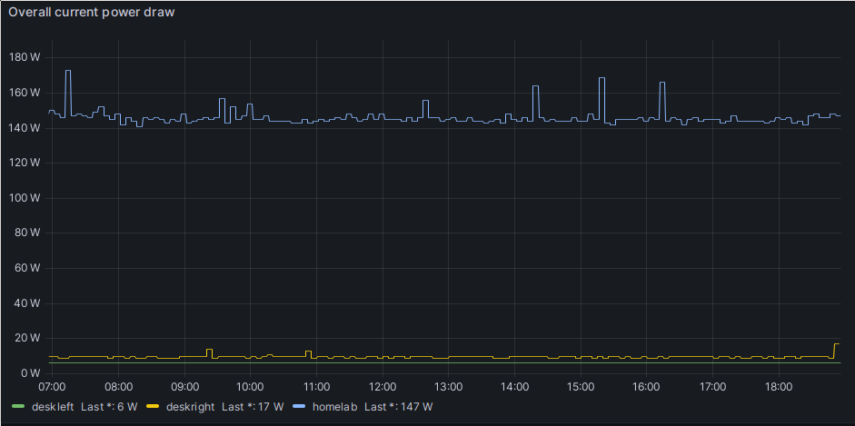
The plot showing current power draw of my setup. The homelab curve is my entire Homelab setup, while deskright and deskleft are the power strips powering the rest of my desk, e.g. my desktop, WiFi AP etc.
This is the most boring plot, from the PoV of PromQL, and at the same time the
one I look at the most. The PromQL query is just mqtt_power.
Total power draw in kWh
The next panel has an at least a bit more complex query config. It shows the total power draw in kWh, for all three plugs in my system, for both the current day, and the previous day.
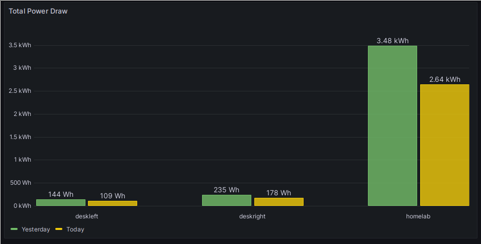
Total Power Draw plot. Notably, this screenshot was taken for a day where I wasn’t home at all.
As I noted, the config is a bit more interesting here. First of all, there are
two PromQL queries for this plot, one on mqtt_yesterday_pwr and one on
mqtt_today_pwr. The type of the plot is bar chart. The X axis is configured
to go over the sensor label. This label is set to the different names for my
plugs, which in turn are named for the location they’re plugged in.
The problem with this plot was that I wanted the two different metrics, the
total consumption for today and yesterday, as two separate bars for each of
the labels. After some trial and error, I figured out that I can do it in
Grafana by using “Transforms”. I’m using two of them. The more important one
is the Join by labels transform. See the Grafana docs here. I’m joining on the _name_
of the sensor label. This way, I end up with the values grouped by sensor.
Then I’m using an Organize fields transform, to rename mqtt_yesterday_pwr
and mqtt_today_pwr to Yesterday and Today respectively. This makes the
labels a bit nicer.
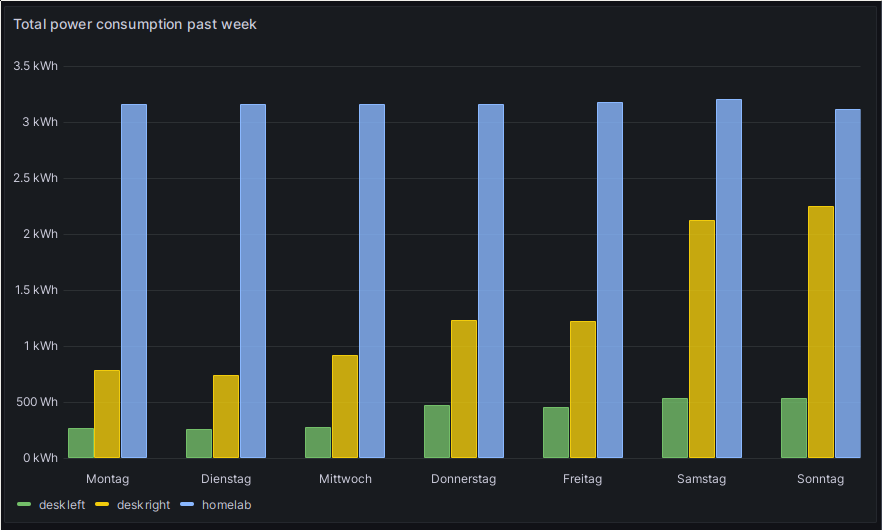
Power consumption per day over one week
This is the one plot which does not really work as intended. The idea was to show the values for total power draw for all three plugs per day for the past week, to get an overview of how the consumption is developing.
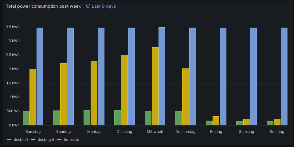
Total Power Draw plot. Notably, this screenshot was taken for a day where I wasn’t home at all.
This plot was the most complicated one, and it still does not work right.
Having a look at the screenshot above, note how both the deskleft and deskright
plots get considerably lower starting on Friday? That’s wrong. The week that’s
shown here was a vacation week for me, which is why the values for deskleft
and deskright got so high - those plugs are measuring the power consumption of
my desktop machine, including screens. And on Thursday (Donnerstag), I left
very early to visit some friends and family, where I wasn’t home at all.
But Thursday is still very high - which is because those bars are actually the
values for Wednesday (Mittwoch), not the ones for Thursday. So something is
still wrong in my config.
Still, I want to show you a little bit of what’s going on in the Grafana config for this particular plot.
First, the PromQL query:
max_over_time(mqtt_today_pwr[24h] offset -24h)
This takes the 24h long intervals (meaning all data points in that interval),
and takes the maximum over it - which, because the daily value resets at
midnight, is the final value of that day. The -24h offset is needed to make
sure that you actually get a value from the previous day - not the current day.
The real “magic” here happens in the Grafana query options though. Here, I configured the “Relative time” field to “8d”, which gives me the entire past week.
I’m not 100% sure which configuration is throwing the daily alignment out of
whack here.
I think something is wrong with my assumption that the 24h offset together
with max_over_time guarantees that I get the max value for each day.
Some interesting data points
Before finishing the article, I want to show off a couple of interesting plots.
This first one showed an interesting change: I switched off a VM, which served as a Nomad worker, on my x86 server. The server kept running, and was at that point still running two Ceph nodes. But it was no longer running any Nomad workloads. All of the workloads still ran, just now on Raspberry Pis instead of a VM on my x86 server.
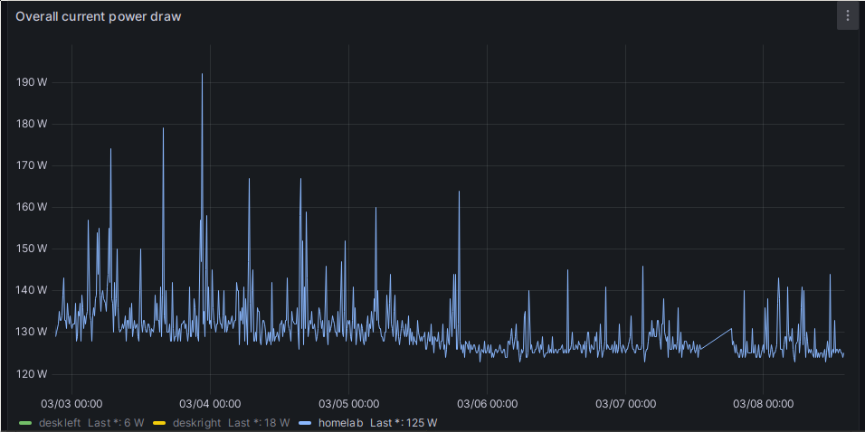
Plot showing homelab power consumption. Notably, the floor drops from 130W to 125W around March 5th.
This next one mostly shows how expensive running a Gentoo desktop is. I think I should switch to Ubuntu or something like it, for the sake of the environment. 😅
Plot showing my desktop’s power consumption during a Gentoo Linux world update.
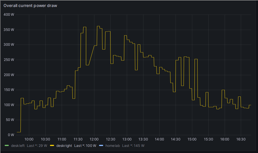
In the same vain, gaming is also damned expensive. Here is my desktop’s power consumption during a night of Anno 1800. You can even see where I hit the pause button to grab something to drink or go for a smoke.
Plot showing my desktop’s power consumption while playing Anno 18:00.
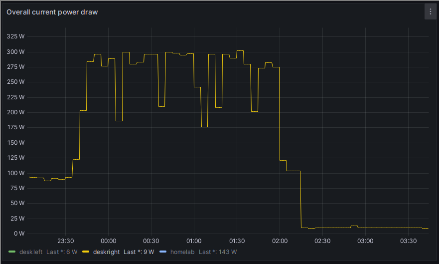
Another one I found interesting is the consumption while I’m working from home. You can even see where I got coffee or went for a smoke and Windows put my screens in stand-by.
Plot showing the power consumption during a Work from Home day.
Another PoV is the daily total consumption for that week, where I was working from home Thursday and Friday. On both days, I used approximately 430 Wh more in electricity than on the other days, where I was working from the office.
Plot showing my power consumption during a week where I worked from home on Thursday and Friday.
To be honest, this project wasn’t very much about controlling/reducing my power consumption. The switch to mostly Raspberry Pis for the Homelab was planned before I ever started measuring the lab’s power consumption. But I mostly wanted it to figure out whether replacing my one x86 machine with all my current gear would reduce my electricity needs. It turns out it did not.
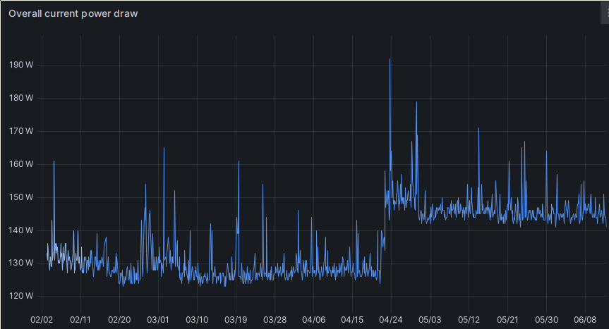
Plot showing my homelab’s power consumption from when measurements started until the time of writing this article.
The sudden jump in power consumption at the end of April was when I added another x86 machine as a ceph host, and the slight drop shortly thereafter was when I finally switched off my original home server.
Ah well, the primary goal was high availability anyway. 😉